statsmodels review
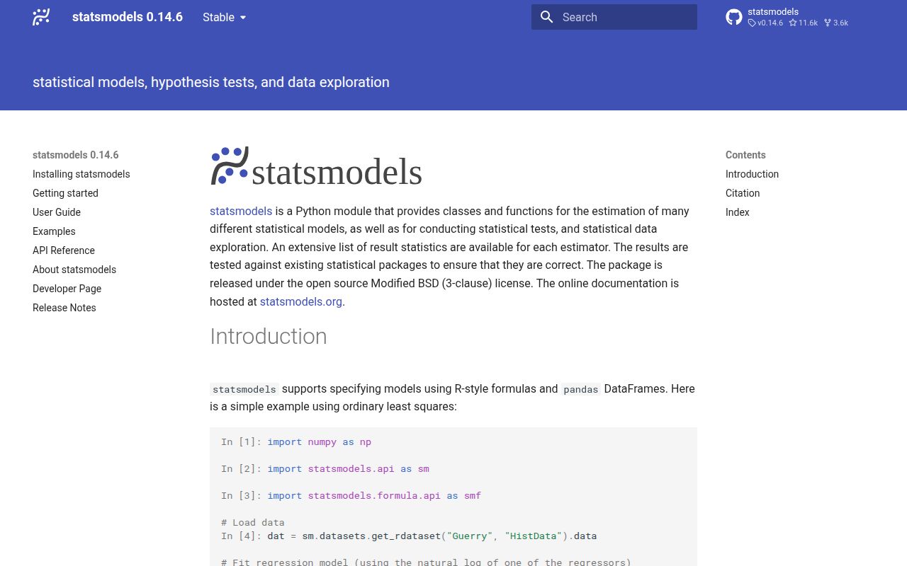
statsmodels fits statistical models and reports inference, not only predictions. Its regression, generalized linear, discrete-choice, mixed-effects, survival, multivariate, and time-series families expose coefficients, covariance estimates, hypothesis tests, confidence intervals, likelihood criteria, residual diagnostics, and printable summaries. You can pass arrays through `statsmodels.api` or use Patsy formulas such as `spend ~ income + C(region)`. Version 0.14.6 is a maintenance release aimed at compatibility with recent NumPy changes. Our install pulled a large scientific stack, included compiled extensions, and did not include a `py.typed` marker.
statsmodels is the Python choice when a model must support inference and diagnostics instead of ending at `predict()`. Accept its 248 MB measured environment and API quirks only when those statistical outputs are part of the deliverable.
We installed it
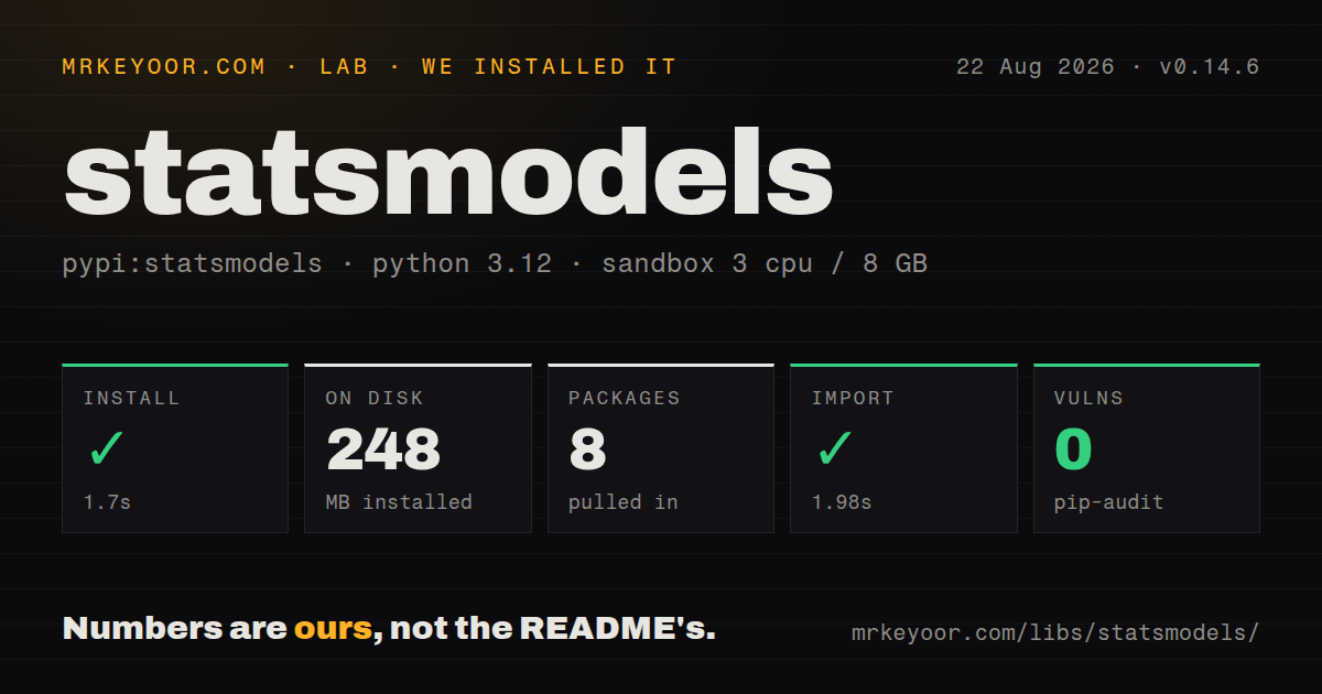
| Install | ✓ · 1.7s | 8 packages on disk · 248 MB |
| Import | ✓ | import statsmodels in 1.98s · compiled extensions · requires Python >=3.9 |
| Known vulns | 0 | (pip-audit) |
Answers from our run
Does statsmodels install cleanly?
Yes. In a fresh container with an empty cache, pip install statsmodels finished in 2 seconds, leaving 8 packages and 248 MB on disk. pip-audit reported no known vulnerabilities.
What does statsmodels need to run?
Python >=3.9, and a platform wheel with compiled extensions. In our run import statsmodels succeeded in 1.98s.
statsmodels or scikit-learn: which should you use?
scikit-learn: Use it for prediction pipelines, cross-validation, preprocessing, and regularized estimator selection. statsmodels is the Python choice when a model must support inference and diagnostics instead of ending at predict().
When should you not use statsmodels?
The main target is out-of-sample prediction with preprocessing pipelines, cross-validation, and model selection. Scikit-learn owns that workflow
Use it if
- The result must explain coefficient uncertainty with standard errors, confidence intervals, p-values, and diagnostic tests
- An analysis is moving from R or Stata and formula syntax with categorical contrasts will reduce translation work
- You need ARIMA, state-space, vector autoregression, seasonal decomposition, or unit-root tests in one Python package
- Regression needs clustered or heteroskedasticity-consistent covariance estimates rather than only point predictions
- The main target is out-of-sample prediction with preprocessing pipelines, cross-validation, and model selection. Scikit-learn owns that workflow
- You need a few standalone tests or distributions. SciPy avoids the 248 MB environment we measured for the full statsmodels install
- Panel data, fixed effects, or instrumental variables are central. Some related code remains in the statsmodels sandbox, which the project says is not production ready; `linearmodels` is built for those models
- Bayesian posterior inference and user-defined priors are required. PyMC supplies sampling and posterior diagnostics that classical statsmodels fits do not
- Static typing must be complete across the public API. Our installed-package check found compiled extensions and no `py.typed` marker
Setup reality
We installed statsmodels 0.14.6 in a fresh Python 3.12 Bookworm container. pip succeeded in 1.7 seconds, leaving 8 packages and 248 MB on disk. Package metadata lists 28 direct dependencies and requires Python 3.9 or newer. The distribution includes compiled .so extensions and no py.typed marker. import statsmodels completed in 1.98 seconds. pip-audit found no known vulnerabilities in the resolved environment. This is the heaviest install in this batch by a wide margin.
Common platforms receive wheels. Unsupported platforms or a new Python and NumPy combination may need a compiler, Cython, and scientific build headers because statsmodels contains native extensions. Version 0.14.6 specifically updates compatibility for recent NumPy changes, so keep NumPy, SciPy, pandas, Patsy, and statsmodels together in environment tests. Import annotations may exist in places, yet the missing typing marker means strict checkers cannot assume the installed package is fully typed.
The array API does not add an intercept. Call sm.add_constant(X) when the model needs one; otherwise OLS fits through the origin and even reports a different form of R-squared. Formula models include an intercept unless the formula removes it. Missing-data defaults are another quiet trap: clean the frame or pass missing='drop' or missing='raise' rather than accepting a result table filled with NaNs. Preserve row alignment when clusters, weights, or offsets come from separate Series.
Formulas are parsed by Patsy, which expands categorical variables and interactions and evaluates transforms. That convenience can make prediction fail when new data contains unseen levels or lacks the original column names. Time-series forecasts need a dated index with a frequency if returned predictions should carry dates. Some modules live under sandbox; the project explicitly says that area is in varying stages of development and is unsuitable as a production guarantee.
Patterns
Fit OLS with an explicit intercept fit-ols-arrays
import statsmodels.api as sm

X = sm.add_constant(df[['income', 'age']])
y = df['spend']
fit = sm.OLS(y, X, missing='raise').fit()
print(fit.summary())
The array API does not add a constant. `missing='raise'` catches NaNs before they turn the results into NaNs.
Fit categorical terms with a formula fit-ols-formula
import statsmodels.formula.api as smf

fit = smf.ols(
    'spend ~ income + age + C(region) + income:age',
    data=df,
).fit()
Formulas add an intercept by default and Patsy chooses a reference category for `C(region)`.
Report logistic odds ratios logistic-regression
import numpy as np
import statsmodels.formula.api as smf

fit = smf.logit('converted ~ visits + C(plan)', data=df).fit()
odds = np.exp(fit.params)
intervals = np.exp(fit.conf_int())
`predict()` returns probabilities. Perfect separation may raise or produce huge unstable coefficients.
Use HC3 standard errors hc3-covariance
fit = smf.ols('spend ~ income + age', data=df).fit(cov_type='HC3')
print(fit.params)
print(fit.bse)
The covariance choice changes standard errors, test statistics, and intervals, while coefficient estimates remain the same.
Cluster standard errors by store clustered-errors
fit = smf.ols('spend ~ income', data=df).fit(
    cov_type='cluster',
    cov_kwds={'groups': df.loc[df.index, 'store_id']},
)
The group vector must align exactly with rows retained by the model after missing-data handling.
Return mean and observation intervals prediction-interval
new = pd.DataFrame({'income': [50000, 90000], 'age': [30, 45]})
frame = fit.get_prediction(new).summary_frame(alpha=0.05)
print(frame[['mean', 'mean_ci_lower', 'mean_ci_upper', 'obs_ci_lower', 'obs_ci_upper']])
Observation intervals describe individual future values and are wider than intervals for the conditional mean.
Fit counts with an exposure offset poisson-offset
import numpy as np
import statsmodels.api as sm

X = sm.add_constant(df[['promo', 'weekend']])
fit = sm.GLM(
    df['orders'], X, family=sm.families.Poisson(),
    offset=np.log(df['visits']),
).fit()
The offset is on the link scale. Check overdispersion before trusting Poisson standard errors.
Forecast a dated ARIMA series arima-forecast
from statsmodels.tsa.arima.model import ARIMA

series = df.set_index('date')['sales'].asfreq('D')
fit = ARIMA(series, order=(2, 1, 2), seasonal_order=(1, 0, 1, 7)).fit()
forecast = fit.get_forecast(steps=14)
print(forecast.conf_int())
Use the current `tsa.arima.model` path. A regular index frequency keeps dates on forecast output.
Separate trend and seasonality stl-decompose
from statsmodels.tsa.seasonal import STL

result = STL(series, period=7, seasonal=13, robust=True).fit()
trend = result.trend
seasonal = result.seasonal
remainder = result.resid
`period` counts observations, and the seasonal smoother length must be an odd integer of at least 7.
Test residual variance and autocorrelation diagnose-residuals
from statsmodels.stats.diagnostic import het_breuschpagan
from statsmodels.stats.stattools import durbin_watson

lm, lm_pvalue, fvalue, f_pvalue = het_breuschpagan(fit.resid, fit.model.exog)
dw = durbin_watson(fit.resid)
A diagnostic p-value identifies evidence against an assumption; it does not select the correct replacement model by itself.
Compare ADF and KPSS stationarity tests unit-root-tests
from statsmodels.tsa.stattools import adfuller, kpss

adf_p = adfuller(series.dropna())[1]
kpss_p = kpss(series.dropna(), regression='c')[1]
print({'adf_p': adf_p, 'kpss_p': kpss_p})
ADF uses a unit-root null, while KPSS uses a stationarity null. Read the two p-values under their different hypotheses.
Build a coefficient DataFrame tidy-coefficients
interval = fit.conf_int().rename(columns={0: 'lower', 1: 'upper'})
tidy = pd.DataFrame({
    'coefficient': fit.params,
    'std_error': fit.bse,
    'p_value': fit.pvalues,
}).join(interval)
Use result attributes instead of parsing the formatted text returned by `summary()`.
Alternatives
| Package | Registry | Pick it when |
|---|---|---|
| scikit-learn | PyPI | Use it for prediction pipelines, cross-validation, preprocessing, and regularized estimator selection. |
| scipy | PyPI | Use it for distributions, optimization, and standalone statistical tests without a full model-results framework. |
| linearmodels | PyPI | Use it for panel estimators, fixed effects, instrumental variables, 2SLS, GMM, and system regression. |
| pymc | PyPI | Use it when priors, posterior distributions, and sampling diagnostics define the analysis. |
More data guides
numpy · fsspec · pandas · sqlalchemy · pyarrow · lxml · the whole shelf →
How this guide is made: grounded in the library's documentation, release notes, changelog, and issue history, on a fixed rubric — not a hands-on install of every release. The 50 most-downloaded entries are additionally install-verified in clean containers. Corrections: contact the desk.