scipy review
SciPy 1.18.1 supplies numerical algorithms that operate on NumPy arrays, including optimization, integration, interpolation, statistics, signal processing, sparse linear algebra, spatial searches, special functions, image operations, and FFTs. Version 1.18.1 adds no new user-facing functions over 1.18.0; it is a corrective release that publishes Python 3.15 wheels and raises the source-build GCC minimum to 10.3. The 1.18 series also expands batched linear algebra, ILP64 BLAS work, Array API coverage, FFT backends, and smoothing methods.
SciPy 1.18.1 installed in 0.9 seconds but consumed 168 MB in our sandbox, a good trade only when the application needs its compiled numerical methods rather than basic NumPy operations. Confirm wheel support, convergence signals, and backend compatibility before putting it on a constrained target.
We installed it
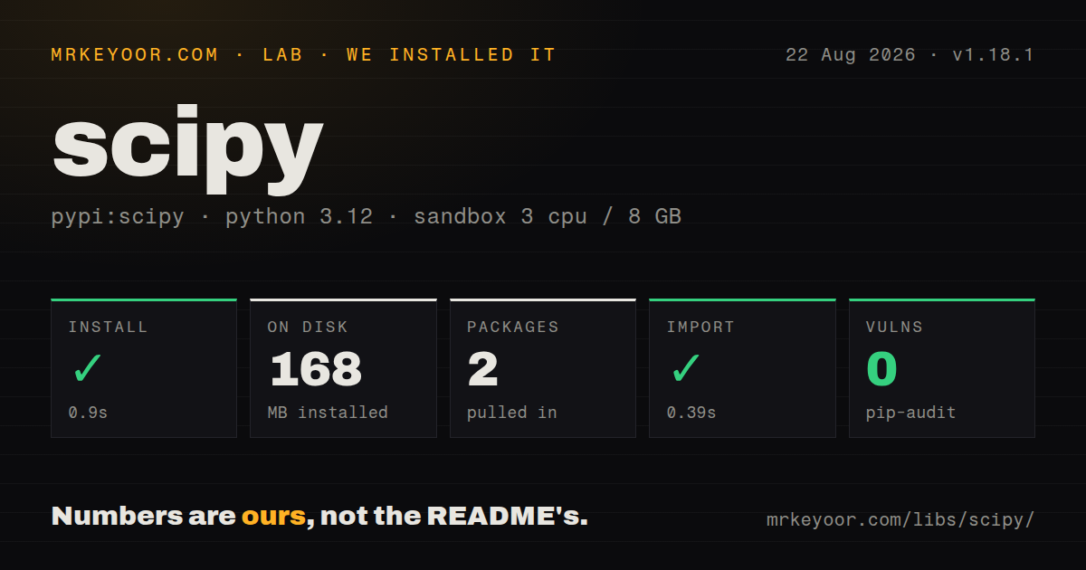
| Install | ✓ · 0.9s | 2 packages on disk · 168 MB |
| Import | ✓ | import scipy in 0.39s · compiled extensions · requires Python >=3.12 |
| Known vulns | 0 | (pip-audit) |
Answers from our run
Does scipy install cleanly?
Yes. In a fresh container with an empty cache, pip install scipy finished in 0.9s, leaving 2 packages and 168 MB on disk. pip-audit reported no known vulnerabilities.
What does scipy need to run?
Python >=3.12, and a platform wheel with compiled extensions. In our run import scipy succeeded in 0.39s.
scipy or numpy: which should you use?
numpy: Use it when arrays, vectorization, dense linear algebra, and basic transforms cover the computation. SciPy 1.18.1 installed in 0.9 seconds but consumed 168 MB in our sandbox, a good trade only when the application needs its compiled numerical methods rather than basic NumPy operations.
When should you not use scipy?
If arrays, broadcasting, basic FFTs, and dense linear algebra are enough, NumPy avoids the 168 MB environment measured for SciPy.
Discussed on
- hnSciPy builds for Python 3.12 on Windows are a minor miracle475 points
- hnScipy Lecture Notes – Learn numerics, science, and data with Python473 points
- hnSciPy 1.0: fundamental algorithms for scientific computing in Python387 points
- hnCuPy: NumPy and SciPy for GPU377 points
- hnScipy 1.0 released370 points
Use it if
- A NumPy application needs established solvers, distributions, optimizers, filters, interpolation, transforms, or integration routines.
- Compiled implementations of standard numerical algorithms are preferable to maintaining equivalent Python code.
- One analysis crosses scientific domains and benefits from common ndarray and result-object conventions.
- Sparse matrices, sparse arrays, and sparse solvers must live beside dense NumPy operations.
- If arrays, broadcasting, basic FFTs, and dense linear algebra are enough, NumPy avoids the 168 MB environment measured for SciPy.
- SciPy 1.18.1 requires Python 3.12 or newer, so it cannot fit a service pinned to 3.11 or below.
- A platform without a compatible wheel needs a serious native build setup, including GCC 10.3+, C and C++ tooling, BLAS, and LAPACK.
- Choose JAX or a framework-native numerical library when automatic differentiation, accelerators, and one consistent device execution model are central.
- Our distribution check found no `py.typed` marker, which may disqualify SciPy where installed-package typing metadata is mandatory.
Setup reality
Our SciPy 1.18.1 install used a wheel and completed in 0.9 seconds in a fresh Python 3.12 Bookworm container. The environment held 2 packages and occupied 168 MB. pip-audit found 0 known vulnerabilities. Package metadata contains 40 dependency entries, requires Python 3.12+, and ships compiled .so extensions. import scipy succeeded in 0.39 seconds, while our inspection found no py.typed marker.
SciPy needs no credentials or application config. Wheel availability is the deciding installation detail. Building version 1.18.1 from source requires GCC 10.3 or newer plus the native numerical toolchain. BLAS and LAPACK selection affects speed, supported integer widths, and redistribution. The measured binary includes license notices for SciPy, OpenBLAS, LAPACK, GCC runtime libraries, and libquadmath, so vendors should retain the wheel's notices rather than reducing them to one label.
Import routines from submodules such as scipy.optimize and scipy.stats; the top-level name is not a flat catalog. Many calls return result objects whose status, convergence flag, or warning matters as much as the computed array. A populated result.x does not mean an optimizer succeeded. Sparse arrays and older sparse matrices differ in multiplication and shape behavior, so choose one model explicitly in new code.
Numerical defaults encode assumptions about scale and data. Set bounds, axes, tolerances, missing-value behavior, and random generators where those choices affect conclusions. SciPy 1.18 broadens batched operations and experimental Array API paths, but backend coverage is still per function. Test the exact call before assuming a CuPy, JAX, or other array can travel through an entire pipeline without returning to NumPy.
Patterns
Minimize with explicit bounds minimize-objective
from scipy.optimize import minimize; result = minimize(loss, x0=[0.0, 0.0], bounds=[(-2, 2), (-2, 2)])Read `result.success` and `result.message` before trusting the returned parameters. A result array exists even after some failures.
Integrate an initial-value problem solve-initial-value-problem
from scipy.integrate import solve_ivp; solution = solve_ivp(rhs, (0, 10), y0=[1.0], rtol=1e-7, atol=1e-9)Tolerances must match the scale of the state. Check `solution.success` and inspect any event or step failures.
Compare two independent samples run-hypothesis-test
from scipy.stats import mannwhitneyu; result = mannwhitneyu(a, b, alternative='two-sided')The study design and sampling process decide whether this nonparametric test and its assumptions make sense.
Filter offline data without phase shift filter-signal
from scipy.signal import butter, sosfiltfilt; sos = butter(4, 20, btype='low', fs=rate, output='sos'); filtered = sosfiltfilt(sos, samples)`sosfiltfilt` reads future samples, so this result cannot be reproduced by a causal live filter.
Interpolate without overshoot interpolate-points
from scipy.interpolate import PchipInterpolator; curve = PchipInterpolator(x, y, extrapolate=False); output = curve(query_x)Input `x` values must be unique and ordered. With extrapolation disabled, queries beyond the data range return NaN.
Solve a sparse system solve-sparse-system
from scipy.sparse import csr_array; from scipy.sparse.linalg import spsolve; x = spsolve(csr_array(matrix), b)Check the residual and warnings because singular or poorly conditioned matrices can still produce numeric output.
Find nearby points with a KD-tree find-nearest-neighbors
from scipy.spatial import cKDTree; distance, index = cKDTree(points).query(targets, k=3)Distance depends on coordinate scale. Normalize dimensions first when their units should contribute comparably.
Transform a real-valued signal compute-fast-fourier-transform
from scipy.fft import rfft, rfftfreq; spectrum = rfft(samples); frequencies = rfftfreq(len(samples), d=1 / rate)Detrending and windowing are separate choices; both can materially change how the frequency bins are interpreted.
Fit parameters to a nonlinear curve fit-nonlinear-curve
from scipy.optimize import curve_fit

params, covariance = curve_fit(model, x, y, p0=[1.0, 0.1], bounds=(0, float('inf')))
errors = covariance.diagonal() ** 0.5
Parameter errors assume the fitted model and data conditions justify the covariance estimate. Inspect residuals instead of reporting the diagonal alone.
Apply a Gaussian image filter smooth-image
from scipy.ndimage import gaussian_filter

smoothed = gaussian_filter(image, sigma=(1.5, 1.5), mode='reflect')
`sigma` is measured in pixels along each axis. Channel dimensions need a zero sigma or separate handling to avoid mixing colors.
Evaluate a stable logistic function stable-logistic-function
from scipy.special import expit

probability = expit(logits)
`expit` avoids the direct exponential expression that can overflow for large negative inputs.
Solve a dense linear equation solve-dense-system
from scipy.linalg import solve

x = solve(a, b, assume_a='pos')
Set `assume_a='pos'` only for a positive-definite matrix. A wrong structural promise can select an unsuitable solver.
Alternatives
| Package | Registry | Pick it when |
|---|---|---|
| numpy | PyPI | Use it when arrays, vectorization, dense linear algebra, and basic transforms cover the computation. |
| statsmodels | PyPI | Use it for fitted statistical models, inference summaries, diagnostics, and econometric workflows. |
| scikit-learn | PyPI | Use it for estimators, preprocessing, model selection, and machine-learning pipelines built on the scientific stack. |
More data guides
numpy · fsspec · pandas · pyarrow · sqlalchemy · s3fs · the whole shelf →
How this guide is made: grounded in the library's documentation, release notes, changelog, and issue history, on a fixed rubric — not a hands-on install of every release. The 50 most-downloaded entries are additionally install-verified in clean containers. Corrections: contact the desk.