geopandas review
GeoPandas 1.1.4 adds vector geometry to pandas tables. A `GeoDataFrame` holds ordinary columns plus an active Shapely geometry column and a coordinate reference system, then supplies spatial joins, overlays, clipping, projection, file I/O, PostGIS I/O, and maps. It is for points, lines, and polygons, not raster pixels. The 1.1.4 patch hardens `to_postgis` against SQL injection and fixes point sampling order, categorical legends in `explore()`, and empty-input handling in `overlay()`.
GeoPandas 1.1.4 imported in 1.72 seconds after our 1.3-second install, but the fresh environment occupied 246 MB across 10 packages. Install it for in-memory vector analysis that already fits the pandas model; choose a raster tool, spatial database, or partitioned engine when pixels, scale, or concurrency define the problem.
We installed it
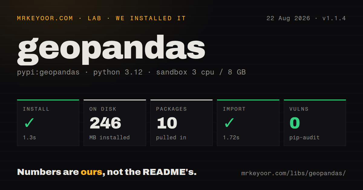
| Install | ✓ · 1.3s | 10 packages on disk · 246 MB |
| Import | ✓ | import geopandas in 1.72s · pure Python · requires Python >=3.10 |
| Known vulns | 0 | (pip-audit) |
Answers from our run
Does geopandas install cleanly?
Yes. In a fresh container with an empty cache, pip install geopandas finished in 1 seconds, leaving 10 packages and 246 MB on disk. pip-audit reported no known vulnerabilities.
What does geopandas need to run?
Python >=3.10, and nothing compiled: it is pure Python. In our run import geopandas succeeded in 1.72s.
geopandas or shapely: which should you use?
shapely: Use it when geometry construction and predicates are enough and a pandas table adds no value. GeoPandas 1.1.4 imported in 1.72 seconds after our 1.3-second install, but the fresh environment occupied 246 MB across 10 packages.
When should you not use geopandas?
The source is satellite imagery, elevation tiles, or another raster grid. Rasterio or rioxarray models pixels directly, while GeoPandas models vector features.
Use it if
- Your existing pandas analysis needs point, line, or polygon columns with spatial predicates and joins.
- A notebook or batch job must clip, dissolve, overlay, reproject, or map vector features.
- You exchange GeoPackage, Shapefile, GeoJSON, GeoParquet, or PostGIS data and want one table-shaped interface.
- The dataset fits in memory and one Python process is an acceptable execution model.
- The source is satellite imagery, elevation tiles, or another raster grid. Rasterio or rioxarray models pixels directly, while GeoPandas models vector features.
- The working set exceeds one machine's memory. GeoPandas inherits pandas' eager in-memory behavior; PostGIS, DuckDB Spatial, or Dask-GeoPandas can move or partition the work.
- You cannot manage coordinate systems explicitly. The README says operations are Cartesian and does not enforce matching coordinates, so distance and area on longitude and latitude can look plausible while being wrong.
- A 246 MB fresh environment is too expensive for the job. Our install pulled 10 packages even though the GeoPandas wheel itself is pure Python.
- Static typing must be declared complete by the package. Our 1.1.4 install did not include `py.typed`, so a strict checker may not treat all inline annotations as supported public typing.
Setup reality
We installed GeoPandas 1.1.4 in 1.3 seconds in a fresh Python 3.12 Bookworm sandbox. The environment contained 10 packages and occupied 246 MB. The package declares 23 dependency entries, requires Python 3.10 or newer, and its own wheel is pure Python. import geopandas worked and took 1.72 seconds. pip-audit reported 0 known vulnerabilities. We found no py.typed marker, and the package metadata did not expose a license value in our measurement.
The one-line pip command brings in the compiled geospatial stack through dependencies such as Shapely, pyproj, and pyogrio. Common wheels avoid a compiler. Less common platforms or source builds can expose GEOS, PROJ, and GDAL compatibility work, which is why the project points difficult installs toward conda. Plotting, interactive maps, database access, and Parquet add optional packages; do not assume pip install geopandas includes Matplotlib, Folium, SQLAlchemy, a PostgreSQL driver, or PyArrow.
CRS handling is the first runtime trap. set_crs() labels the coordinates already present, while to_crs() calculates new coordinates. Area, distance, buffering, and nearest joins are Cartesian. Project longitude and latitude into a suitable local CRS before measuring. Both sides of a binary operation need compatible coordinate systems because GeoPandas 1.1.4 still does not enforce that match for every operation.
Spatial joins and overlays can multiply rows when features cross several partners, and geometry repair can turn a Polygon into a MultiPolygon or GeometryCollection. Check output counts, geometry types, empty values, and validity before writing. Version 1.1.4 specifically improves overlay(..., keep_geom_type=...) with empty input and hardens to_postgis, but connection privileges, transactions, table replacement policy, and secret handling remain application decisions.
Patterns
Read chosen columns from a GeoPackage read-vector-layer
import geopandas as gpd

parcels = gpd.read_file(
    'parcels.gpkg',
    layer='parcels',
    columns=['parcel_id', 'owner', 'geometry'],
)
print(parcels.crs)
Inspect `crs` as soon as the layer loads. A missing or incorrect label invalidates later projection, distance, and area work.
Create points from longitude and latitude build-point-frame
import pandas as pd
import geopandas as gpd

rows = pd.DataFrame({'name': ['Oslo'], 'lon': [10.7522], 'lat': [59.9139]})
places = gpd.GeoDataFrame(
    rows,
    geometry=gpd.points_from_xy(rows.lon, rows.lat),
    crs='EPSG:4326',
)
`points_from_xy` takes x before y. For EPSG:4326 that means longitude before latitude.
Transform coordinates before measuring project-for-meters
metric = places.to_crs(places.estimate_utm_crs())
metric['buffer_250m'] = metric.geometry.buffer(250)
metric['area_m2'] = metric['buffer_250m'].area
`to_crs()` transforms coordinates. `set_crs()` only assigns a label and must not be used as a shortcut for metric calculations.
Attach district data to points join-points-to-polygons
districts = districts.to_crs(places.crs)
joined = gpd.sjoin(
    places,
    districts[['district_id', 'geometry']],
    how='left',
    predicate='within',
).drop(columns='index_right')
A boundary point is not `within` its polygon. Use `intersects` if boundary matches should count, and expect extra rows if polygons overlap.
Find a nearby station with a distance limit join-nearest-feature
local_crs = addresses.estimate_utm_crs()
result = gpd.sjoin_nearest(
    addresses.to_crs(local_crs),
    stations.to_crs(local_crs),
    how='left',
    max_distance=5_000,
    distance_col='distance_m',
)
The 5,000-unit limit is only 5 km when the chosen projected CRS uses meters. Nearest calculations are Cartesian.
Clip roads to a city boundary clip-to-boundary
city = city.to_crs(roads.crs)
inside = gpd.clip(roads, city)
inside = inside.explode(index_parts=False).reset_index(drop=True)
Clipping may produce empty, multipart, or changed geometry types. Check the result before writing a format with a fixed geometry schema.
Overlay parcel and zone polygons intersect-polygons
zones = zones.to_crs(parcels.crs)
crossings = gpd.overlay(
    parcels[['parcel_id', 'geometry']],
    zones[['zone_id', 'geometry']],
    how='intersection',
    keep_geom_type=True,
)
One parcel can create several output rows. GeoPandas 1.1.4 fixes empty-input handling with `keep_geom_type`, but row-count validation is still required.
Dissolve county polygons into regions merge-by-region
regions = counties.dissolve(
    by='region',
    aggfunc={'population': 'sum', 'income': 'mean'},
    as_index=False,
)
`dissolve` unions geometry and aggregates attributes. Specify an aggregation for every non-geometry column you intend to retain.
Repair invalid features and inspect type changes repair-invalid-geometry
bad = ~features.geometry.is_valid
features.loc[bad, 'geometry'] = features.loc[bad, 'geometry'].make_valid()
print(features.loc[bad].geom_type.value_counts())
`make_valid()` can return MultiPolygon or GeometryCollection where the input was Polygon. Downstream schemas must accept the repaired types.
Store a GeoDataFrame as GeoParquet write-geoparquet
parcels.to_parquet(
    'parcels.parquet',
    index=False,
    compression='zstd',
)
copy = gpd.read_parquet('parcels.parquet')
Parquet support needs PyArrow. GeoParquet preserves CRS and geometry metadata that ordinary coordinate columns would lose.
Load filtered PostGIS rows read-postgis-query
from sqlalchemy import create_engine, text

engine = create_engine(os.environ['DATABASE_URL'])
sql = text('SELECT id, name, geom FROM places WHERE region_id = :region')
places = gpd.read_postgis(sql, engine, geom_col='geom', params={'region': 7})
SQL access requires SQLAlchemy and a database driver. Parameterize values and filter in the query so one process does not load the full table.
Append features to PostGIS write-postgis-table
features.to_postgis(
    'observations',
    engine,
    schema='gis',
    if_exists='append',
    index=False,
)
GeoPandas 1.1.4 further hardens `to_postgis` against SQL injection. Table privileges and `if_exists` policy still belong in deployment review.
Alternatives
| Package | Registry | Pick it when |
|---|---|---|
| shapely | PyPI | Use it when geometry construction and predicates are enough and a pandas table adds no value. |
| pyogrio | PyPI | Use it when vector file I/O is the job and you prefer a thinner Arrow or NumPy-facing layer. |
| pyproj | PyPI | Use it for coordinate transformations without GeoDataFrame operations or GIS file handling. |
| pandas | PyPI | Use plain pandas when locations are just attributes and no geometric calculation is required. |
More data guides
numpy · fsspec · pandas · sqlalchemy · pyarrow · lxml · the whole shelf →
How this guide is made: grounded in the library's documentation, release notes, changelog, and issue history, on a fixed rubric — not a hands-on install of every release. The 50 most-downloaded entries are additionally install-verified in clean containers. Corrections: contact the desk.