The saved data makes this an audit you can study offline
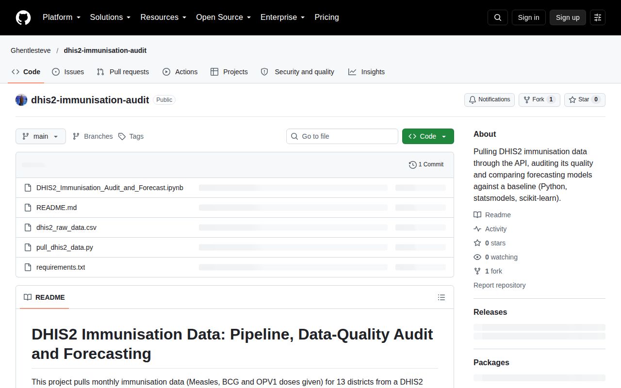
DHIS2 Immunisation Audit starts with a CSV snapshot, so you can examine its reasoning without connecting to a health information server. The notebook looks for missing reports, repeated values and adjacent months that appear swapped. Its best use is teaching an analyst to question a monthly total before fitting a forecasting model. The author explicitly says the source is demo data and the findings do not describe real health trends.
Our checkout had 5 files and about 109 source lines, with the notebook and saved data alongside the pull script. That small surface makes the project approachable for someone who knows pandas and wants a worked example. You can follow an observation back to the underlying rows without first learning a reporting platform. It remains a specific analysis of immunisation indicators, so a different reporting hierarchy will need adaptation. The README sets out the assumptions unusually clearly.
What happened when we ran it
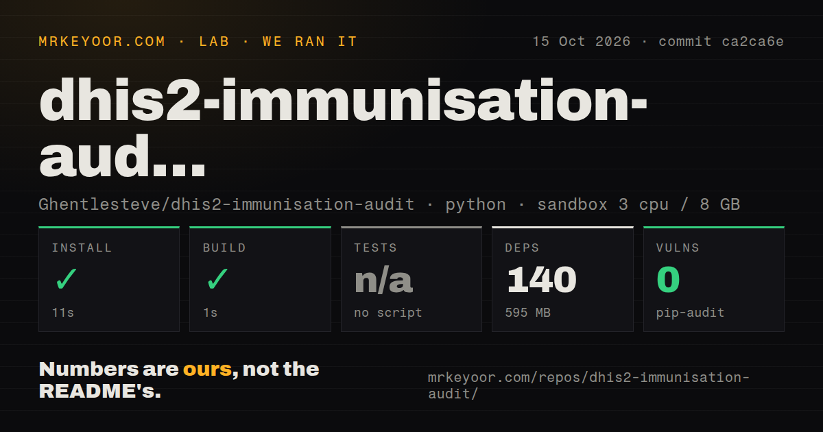
Our sandbox installed commit ca2ca6e in 11 seconds, adding 140 packages and using 595 MB on disk. The build step succeeded in 1 second. The October 15, 2026 run used an unprivileged Debian container with 3 CPUs, 8 GB of RAM and the Python 3.12 Bookworm uv image. These results establish that the measured environment could complete its installation and build steps.
There was no test script or target, so our harness skipped tests. Pip-audit reported 0 known vulnerabilities. The scan also found 0 CI workflow files, no Dockerfile and no tests directory. A successful build therefore supplies little evidence about the notebook's calculations. We did not independently reproduce its forecast errors, validate every chart or confirm that a fresh API pull matches the saved snapshot.
The 595 MB environment is much larger than the 0.5 MB checkout. That is a practical consideration for a classroom or a disposable analysis container, even though installation completed quickly. The README's instructions are short: install the requirements, open the notebook and run the cells in order. Keep the distinction between completing those repository steps and verifying the statistical conclusions, which our lab measurements do not establish.
Missing reports and swapped months get different treatment
The notebook fills missing training observations using the district's history for the same calendar month where available. Where that history is absent, it uses the district's average level with a seasonal pattern across districts. The README labels those filled values as estimates and says they are excluded from forecast scoring. That is useful discipline for an analyst tempted to turn a tidier table into assumed ground truth.
The absence of a test target in our run means these safeguards deserve direct inspection before reuse. In particular, check that your own missing observations remain distinguishable from recorded values after export. The project flags apparently swapped months without correcting them because the data cannot establish their proper order. That restraint is one of its strongest features: it leaves the unresolved question visible for somebody with access to source reports.
The forecast comparison exposes a demo-data problem
The documented comparison pits a seasonal repeat baseline against SARIMA and gradient boosting. The author reports that the baseline wins on this snapshot and connects that result to repeated annual values. The README also identifies a single evaluation window and one forecast indicator as limitations. Treat the comparison as an example of how source-data construction can dominate a modelling result, rather than a general ranking of forecasting methods.
Our 1-second build provides no independent confirmation of that comparison. The README says a rolling evaluation and prediction intervals are next steps, and it lists automated scheduling as future work. Those capabilities are therefore adoption tasks for you. An analyst who needs recurring surveillance should budget for an explicit data contract, recorded run dates and a review process for new exceptions before turning the notebook into a scheduled job.
Refreshing changes both the source and the date window
The notebook defaults to the saved CSV. Setting REFRESH = True enables a new pull, with DHIS2_URL, DHIS2_USER and DHIS2_PASSWORD selecting the server and login. The pull script uses the analytics API and requests district-level organisation units. It searches indicator names, preferring an exact match and otherwise choosing the first available match. Check those selected identifiers before pointing it at another instance.
At 109 source lines, the measured repository is small enough to review that extraction logic directly. Its date helper derives the completed-month window from the current date, so a later refresh will not necessarily analyse the README's original period. Save the extraction date and selected metadata with any new snapshot. The script also prints part of an error response, which deserves inspection before logs from a private server enter a shared notebook or ticket.
A recent push offers no support history to rely on
GitHub records the last push on September 29, 2026, with 0 open issues and PRs and no entries in the issue list we fetched. The latest-release endpoint returned no release. These facts describe a recently updated, small project without visible issue activity, not evidence that it has been abandoned. They also leave you without a demonstrated public support conversation when adapting it to unfamiliar data.
Use this repository when you want to learn an auditable workflow from a saved example. For an operational health reporting platform, DHIS2 itself is the relevant starting point. FG Data Profiling is worth considering for general dataframe reports, although it does not replace this notebook's domain reasoning. Before using this analysis beyond the sample, reproduce one missing-report flag against the raw rows and get the data owner to confirm what the apparent gap means.